# (c) Numerically evaluate the second derivative for f(x)

# Initialize variables for the analysis
t = 3

# Compute the derivative
df2 = 6 * t

print('The second derivative at t = 3 is {}'.format(df2))
The second derivative at t = 3 is 181.1
The first derivative is: \[ \frac{df}{dt} = 3t^2\]
1.2
The second derivative is: \[ \frac{d^2f}{dt^2} = 6t\]
1.3
We calculate the second derivative at time \(t=3\) as follows:
# (c) Numerically evaluate the second derivative for f(x)
# Initialize variables for the analysis
t = 3
# Compute the derivative
df2 = 6 * t
print('The second derivative at t = 3 is {}'.format(df2))The second derivative at t = 3 is 181.4
This derivative, which is the second derivative of distance with respect to time represents the acceleration of the ball in \(m^2\) per second. This shows how quickly the ball is increasing its speed over time.
2.1
Plotting the first derivative of \(f(t)\) for the values \(-2 \leq t \leq 1\)
%config InlineBackend.figure_format = 'retina' # Make clear on high-res screens
import numpy as np
import matplotlib.pyplot as plt

# Create the data to plot
t = np.linspace(-2,2,1000)
f_derivative = 3 * t**2

# Plot the data
fig, ax = plt.subplots(figsize=(5,5))
ax.plot(t,f_derivative, color = 'red')

# Always use X and Y labels. Note that in Python r'string' allows LaTeX to
# interpret the content of the text string
ax.set_xlabel(r'$t$ (seconds)')
ax.set_ylabel(r'Velocity, $\frac{df}{dt}$, (m/s)')
ax.set_xlim([-2,2])
ax.grid('on')
fig.tight_layout()
plt.show()
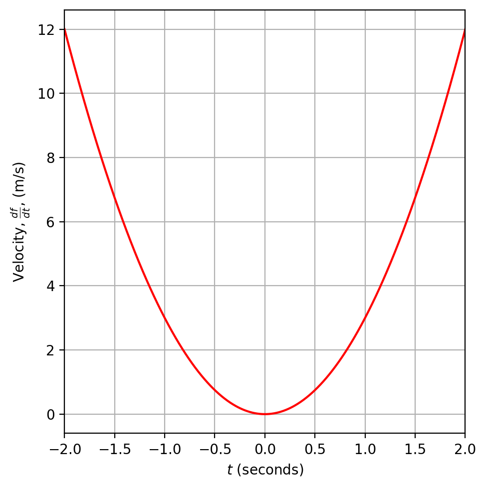
Figure 1. The velocity (first derivative of distance) in meters per second.
2.2
The first derivative of \(f(t)\), which represents distance in meters as a function of time in seconds is velocity, in units of meters per second, as plotted in Figure 1. In this case, that means that at time \(t=2\) the velocity is 12 meters per second.